
Biostatistics Tutorial
Statistics can be defined as the science of collecting, organizing, analyzing and interpreting data - when applied to biological problems, it is known as biostatistics. The role of biostatistics is vital in every stage from research conception to the final analysis. A minimum knowledge of biostatistics is essential to be a successful researcher. This chapter examines basic biostatistical principles and explores their application with relevant examples.
Need for biostatistical tools
Biostatistical tools are necessary in research since it is almost impossible to study an entire population because of the scarcity of resources such as money, time etc or due to a desire to expose only the minimal number of subjects to the risks involved with certain clinical trials. When an entire population cannot be studied, then a part of the population (i.e. sample) is examined.
When the researcher studies the sample and draws inferences about the population, serious errors can result if the sample is not truly representative of the larger population.
Biostatistical tools help the researcher to overcome this bias and help draw valid conclusions about the population with a defined level of confidence. Biostatistics has a role in each phase of the research. Let us start with the first stage of research - planning.
Use of biostatistical tools in planning research
After identifying and defining the problem, the researcher decides on the type of study design to follow. Once the type is determined, the variables have to be identified and classified before proceeding to the next step of developing a hypothesis in the case of experimental study. The variables can be categorized by their nature, type and scales of measurement, i.e. independent or dependent, quantitative or qualitative, types such as nominal, ordinal, interval and ratio scales and so on. The nature of the variables will have a significant effect on data collection and analysis.
Variable classification according to their nature
a. Independent variables: Variables that can either be manipulated by the researcher or which are not outcomes of the study but still affect its results are called independent variables. A good example is age of the subjects, which can be an independent variable that may affect a study outcome variable such as subject survival.
b. Dependent variables: The outcome variables defined as part of the research process are termed dependent variables and these will be affected by the independent variables under study. An example of a dependent variable can be the number of people who developed a particular disease in a cohort study.
Variable classification according to their type
a. Quantitative variables: Variables that can be measured numerically are called quantitative variables. These variables can be further classified as continuous and discrete variables. A continuous variable could take any value in an interval. Examples of continuous data are findings for measurements like body mass, height, blood pressure or serum cholesterol.
Discrete variables will have whole integer values. Examples are the number of hospitalizations per patient in a year or the number of hypoglycemic events recorded in a diabetic patient over 6 months.
b. Qualitative variables: Variables, which cannot be measured numerically, are called qualitative variables. An example is gender.
Variable classification according to the scale of measurement
a. Nominal Scale variables: Nominal scale measurements can only be classified but not put into an order, and mathematical functions cannot be performed on them. Gender is an example for this sort of variable as well.
b. Ordinal Scale Variables: These variables can be put into a definite order, but the difference between two positions in the ordinal scale does not have a quantitative meaning. Essentially, this scale is a form of ranking. An example is the military hierarchy, where a general outranks a colonel who in turn outranks a captain. Though there is a clear series of ranks, the relationship is not numerical.
c. Interval Scale Variables: In an interval measurement scale, one unit on the scale represents the same magnitude of the characteristic being measured across the whole range of the scale, i.e. the intervals between the numbers are equal. However, the ratio between a set of two numbers in the scale are not equal because an interval scale lacks a true zero point.
Temperature in Fahrenheit would be a perfect example for interval scales because though we can add and subtract degrees (70° is 10° warmer than 60°), we cannot multiply values or create ratios (70° is not twice as warm as 35°).
d. Ratio Scale Variables: Ratio scale variables will have all the properties of interval variables with the ratio between two numbers in the ratio scales being identical. Ratio scales have an absolute or zero point. For example, a 100-year old person is indeed twice as old as a 50-year old one.
Statistical Hypothesis
After identifying and defining the variables to be investigated, the researcher has to develop the study hypothesis if conducting an experimental study. Classically, such studies will have two hypotheses. One is a null hypothesis, which is a statement of no effect or no association while the alternative hypothesis is a statement that depicts the researcher's interest or scientific belief.
To illustrate, suppose a researcher wants to test whether a form of chemotherapy for treating small cell lung cancer is more effective than the standard therapy. The researcher can formulate the null and alternative hypothesis as follows:
Null Hypothesis: There is no difference in efficacy between the standard therapy and the new therapy.
Alternative Hypothesis: New therapy is superior to the standard therapy.
Two types of errors can occur while making conclusions regarding the null hypothesis: Type I error and Type II error. A Type I error refers to rejecting the null hypothesis when the null hypothesis is true (false positive). A Type II error refers to accepting the null hypothesis when it is actually false (false negative).
Level of Significance and Power of the Test
The probability of making a Type I error is called level of significance (α). Normally researchers would aim to minimize the probability of making a Type I error. Most researchers will set this probability to 0.05.
The probability of making a Type II error is (β). The power of the study is calculated from (1-β) and is defined as the probability of detecting a real difference when the null hypothesis is false.
These parameters have to be predetermined by the researcher prior to the study to avert the risk of erroneously accepting the null hypothesis (even though it is really false) due to an inadequate sample size that is not enough to detect a true difference.
Once the hypothesis, level of significance and power of the study have been fixed, the researcher can proceed to determine the statistical processes for the proper conduct and analysis of the study.
Sampling
As discussed earlier, the researcher usually draws conclusions about the population from a small part of it – the sample. The information collected from the sample is known as sample statistics which is used to estimate the characteristics of the unknown population i.e. population parameters.
We know that the sample taken from the population should accurately represent the population under study. To get a representative sample, the most important intervention is to select a sample large enough to adequately represent the population. Sadly, researchers have to strike a balance between striving for maximal validity while keeping the cost of the study at a level they can afford!
From what has been stated so far, it can be deduced that the sampling process involves two important aspects. One is deciding the Method of sampling.
Method of Sampling
Method of sampling involves selection of samples from the given population. There are two basic methods in sampling:
a) Probability Sampling
- (i) Simple Random Sampling
- (ii) Stratified Random Sampling
- (iii) Systematic sampling
- (iv) Cluster sampling
b) Non-Probability Sampling
- (i) Judgement sampling
- (ii) Convenience sampling
Determining the sample size is based on a number of issues such as:
- Type of study
- Nature of study i.e. whether estimating parameters or comparing parameters
- Type of sampling method
- Type of analysis used in the study
- Power of the study
- Effect size
- Study budget
- Time factor
It can be readily appreciated that sample size calculation is rather complex. It is always best to consult a statistician for determination of sample size and other challenging biostatistical issues if embarking on a research project.
Data Collection
After determining the sample size the researcher then proceeds to collect data. Data can be gathered through primary or secondary sources.
Primary Sources: Primary sources are original materials collected by the investigator himself. While collecting the primary data, the researcher can use the following methods:
- Personal interview
- Telephone interview
- Face to face administration of questionnaire
- Mailing questionnaire by post
- Mailing questionnaire by email
- Online data collection through websites
Each of the above methods has its advantages and limitations. A rule of thumb is to verify 5% of the data as a quality control measure to validate the data.
Secondary Sources: Secondary data is that which has been collected by individuals or agencies for purposes other than those of our particular research study. Examples of secondary sources are:
- Bibliographies
- Online databases
- Biographies
- Textbooks
- Handbooks and manuals
- Review articles and editorials
Data Compilation & Diagrammatic Analysis
Once the data is collected and validated it can then be compiled. Tabulation is the basic method of compilation. Primary data analysis starts with the diagrammatic and graphical representation of the data. The following are frequently used methods:
A. Histogram
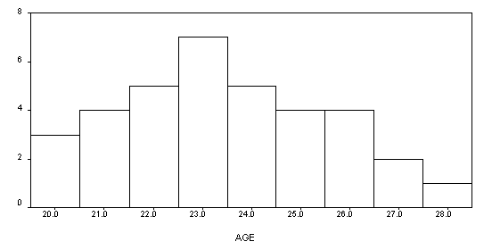
Histograms consist of a series of blocks or bars, each with an area proportional to the frequency. In a histogram the horizontal scale is used for the variable and the vertical scale to show the frequency.
The highest block in a histogram indicates the most frequent values. The lowest blocks show the least frequent values. Where there are no blocks, there are no results that correspond to those values. Blocks of equal height indicate that the values they represent occur in the same frequency.
B. Bar Graph
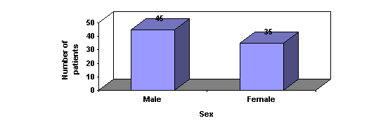
In a simple bar chart, each bar represents a different group of data. Although the bars may be drawn either vertically or horizontally, it is conventional to draw the bars vertically whenever possible. The height or length of the bar is drawn in proportion to the size of the group of data being represented. Unlike a histogram, the bars are drawn separated from one another.
C. Pie Charts
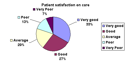
Pie charts, or circle graphs as they are sometimes known, are very different from other types of graphs. They don't use a set of axes to plot points. Pie charts display percentages.
The circle of a pie graph represents 100%. Each portion that takes up space within the circle stands for a part of that 100%. In this way, it is possible to see how something is divided among different groups.
D. Line Graph
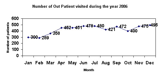
A Line graph is drawn after plotting points on a graph that are then connected by a line. Line graphs are useful to display data trends.
Descriptive Data Analysis
The next stage of data analysis consists of descriptive and inferential data analysis. Descriptive data analysis provides the researcher a basic picture of the problem he is studying. It consists of Measures of Central Tendency, Measures of Dispersion, and Measures of Skewness and Kurtosis.
Measures of Central Tendency
A measure of central tendency is a value that represents a typical or central element of a data set. The important measures of central tendency are Mean, Median, and Mode.
Mean: Mean (average) is the sum of the data entries divided by the number of entries. Sample mean is denoted by X̄ and the population mean is denoted by μ.
Population Mean Formula:

Sample Mean Formula:

Properties of Mean:
- Data possessing an interval scale or a ratio scale, usually have a mean.
- All the values are included in computing the mean.
- A given set of data has a unique mean.
- The mean is affected by unusually large or small data values (known as outliers).
- The arithmetic mean is the only measure of central tendency where the sum of the deviations of each value from the mean is zero.
Median: The median of a data set is the middle data entry when the data set is sorted in order. If the data set contains an even number of elements, the median is the mean of the two middle entries. The median is the most appropriate measure of central tendency to use when the data under consideration are ranked data, rather than quantitative data.
Mode: The mode of a data set is the entry that occurs with the greatest frequency. A set may have no mode or may be bimodal when two entries each occur with the same greatest frequency. The mode is most useful when an important aspect of describing the data involves determining the number of times each value occurs. If the data are qualitative then mode is particularly useful.

Measures of Dispersion
Measures of Dispersion indicate the amount of variation or spread, in a data set. There are four important measures of dispersion: Range, Interquartile Range, Variance, and Standard Deviation.
a) The Range: The range is the difference between the largest and smallest observation. The range is very sensitive to extreme values because it uses only the extreme values on each end of the ordered array. The range completely ignores the distribution of data.
b) The Interquartile Range: The interquartile range (midspread) is the difference between the third and first quartiles (Q3 - Q1). The interquartile range gives the range of the middle 50% of the data, is not affected by extreme values, and ignores the distribution of data within the sample.
c) Variance: The variance is the average of the squared differences between each observation and the mean.
d) Standard Deviation: Standard deviation is the square root of the sample variance. It lends itself to further mathematical analysis in a way that the range cannot because the standard deviation can be used in calculating other statistics. It is worth noting that the standard deviation for nominal or ordinal data cannot be measured because it is not possible to calculate a mean for such data.
Relationships Between Two Variables
Two of the important techniques used to study the relationship between two variables are correlation and regression.
Correlation: Measures association between two variables. In graph form it would be shown as a 'scatter diagram' putting the scores for one variable on the horizontal X axis and the values for the other variable on the vertical Y axis. The pattern shows the strength of the association between the two variables and also whether it is a 'positive' or 'negative' relationship.
- A 'positive' relationship means that as the value on one variable increases so does the value on the other variable.
- A 'negative' relationship means that as the value on one variable increases, the value on the other variable decreases.
Measures of Correlation
There are two measures of correlation. One is Pearson's product-moment correlation (r) and the other is Spearman's rank order co-efficient (rho). Both measures will tell us only how closely the two variables are connected but they cannot tell us whether one causes the other. Correlation values can range from –1 to +1.
Interpretation of correlation values:
- • Equal to 0: No correlation
- • Less than .2: Very low
- • Between .2 and .4: Low
- • Between .41 and .70: Moderate
- • Between .71 and .90: High
- • Over .91: Very high
- • Equal to 1: Perfect correlation

From merely inspecting the diagram we can infer that there is low correlation because the spread is large while the location of the scatter plot towards the upper right tells us that whatever correlation may exist is likely to be positive. The Pearson correlation coefficient for the same data was determined to be 0.196, which confirms a very low positive correlation.
Simple Regression Analysis: It gives the equation of a straight line and enables prediction of one variable value from the other. Normally, the dependent variable is plotted on the Y axis and the independent variable on the X axis. There are 3 major assumptions: first, any value of x and y are normally distributed. Second, the variability of y should be the same for each value of y. Third; the relationship between the two variables is linear.
The equation of a regression line is: y = a + bx where 'a' is the intercept, 'b' is the slope, 'x' is the independent variable and 'y' is the dependent variable. The slope 'b' is sometimes called the regression coefficient and it has the same sign as the correlation co-efficient (r).
Probability & Statistical Distributions
Probability is defined as the likelihood of an event or outcome in a trial: p(A) = (Number of outcomes classified as A) / (Total number of possible outcomes).
Statistical distributions are classified into two categories – discrete and continuous.
Discrete Distributions
Binomial Distribution: It describes the possible number of times that a particular event will occur in a sequence of observations. The event is coded in binary fashion; it may or may not occur. The binomial distribution is used when a researcher is interested in the occurrence of an event, not in its magnitude. For instance, in a clinical trial, a patient may survive or die. The researcher studies only the number of survivors, not how long the patient survives after treatment.
Poisson Distribution: The Poisson distribution is an appropriate model for count data. Examples of such data are mortality of infants in a city, the number of misprints in a book, the number of bacteria on a plate, and the number of activations of a Geiger counter.
Continuous Distributions
Normal Distribution: The normal distribution (also called a Gaussian distribution) is a symmetric, bell-shaped distribution with a single peak. Its peak corresponds to the mean, median, and mode of the distribution. It is characterized by two numbers: Mean gives the location of the peak, and the standard deviation gives the width of the peak.

The 68-95-99.7 Rules for a Normal Distribution:
- About 68.3% of the data in a normally distributed data set will fall within 1 standard deviation of the mean.
- About 95.4% of the data in a normally distributed data set will fall within 2 standard deviations of the mean.
- About 99.7% of the data in a normally distributed data set will fall within 3 standard deviations of the mean.
Inferential Data Analysis
As the researcher draws scientific conclusions from his study using only a sample instead of the whole population, he can justify his conclusion with the help of statistical inference tools. The principal concepts involved in statistical inference are the theory of estimation and hypothesis testing.
Theory of Estimation
Point Estimation: A single value is used to provide the best estimate of the parameter of interest.
Interval Estimation: Interval estimates show the estimate of the parameter and also give an idea of the confidence that the researcher has in that estimate. This leads us to consideration of confidence intervals.
Confidence Interval (CI): A confidence interval estimate of a parameter consists of an interval, along with a probability that the interval contains the unknown parameter. The level of confidence in a confidence interval is a probability that represents the percentage of intervals that will contain the parameter if a large number of repeated samples are obtained. The level of confidence is denoted (1 - α)*100%.
The narrower the width of the confidence interval, the lower is the error of the point estimate it contains. The sample size, sample variance and the level of confidence all affect the width of the confidence interval.
- If the sample size increases it will decrease the width of the confidence interval.
- If the level of confidence increases the width will increase.
- If the variation in sample increases it will increase the width of the confidence interval.
The most commonly used confidence interval is the 95% CI. Increasingly, medical journals and publications require authors to calculate and report the 95% CI wherever appropriate since it gives a measure of the range of effect sizes possible. The term 95% CI means that it is the interval within which we can be 95% sure the true population value lies.
Example: A study is conducted to estimate the average glucose levels in patients admitted with diabetic ketoacidosis. A sample of 100 patients was selected and the mean was found to be 500 mg/dL with a 95% confidence interval of 320-780. This means that there is a 95% chance that the true mean of all patients will lie between 320 and 780.
Hypothesis Testing
The basic concept used in hypothesis testing is that it is far easier to show that something is false than to prove that it is true. This process works with two mutually exclusive and competing hypotheses: the Null Hypothesis (H0) representing a neutral position of no effect, and the Alternative Hypothesis (H1) representing the researcher's interest or scientific belief.
Decision Rule & P-Values: A p-value gives the likelihood of the study effect, given that the null hypothesis is true. The p-value obtained in the study is evaluated against the significance level alpha (α), typically set at 0.05. We can reject H0 if the p-value < α.
Table 1: Step by Step Guide to Applying Hypothesis Testing
| Step | Action Requirement |
|---|---|
| 1 | Formulate a research question |
| 2 | Formulate a research/alternative hypothesis |
| 3 | Formulate the null hypothesis |
| 4 | Collect data |
| 5 | Reference a sampling distribution of the particular statistic assuming that H0 is true |
| 6 | Decide on a significance level (α), typically .05 |
| 7 | Compute the appropriate test statistic |
| 8 | Calculate the p-value |
| 9 | Reject H0 if the p-value is less than the set level of significance, otherwise accept H0 |
Table 2: Statistical Tests at a Glance
| Variable Type | Parameters Tested | Variables Count | Sample Criteria / Assumption | Appropriate Test |
|---|---|---|---|---|
| Ratio Variable | Mean | One | >30 (Large) | Z-test |
| Ratio Variable | Mean | Two | >30 (Large) | Z-test |
| Ratio Variable | Mean | One | <30 (Small) | t-test |
| Ratio Variable | Mean | Two | <30 (Independent) | Independent sample t-test |
| Ratio Variable | Mean (Same Subject) | Two | <30 (Paired) | Paired sample t-test |
| Ratio Variable | Proportion | One | - | Binomial Test |
| Ratio Variable | Proportion | Two | >30 | Z-test for Proportions |
| Ratio Variable | Mean | More than two | >30 | ANOVA |
| Ratio Variable | Mean (Same Subject) | More than two | >30 | Repeated measures ANOVA |
| Nominal/Categorical | Association | Two or more | Expected Frequency ≥ 5 | Chi-square (χ²) Test |
| Ratio Variable | Mean | Two | Normality Assumption Violated | Mann-Whitney U Test |
| Ratio Variable | Mean (Same Subject) | Two | Normality Assumption Violated | Wilcoxon Signed Rank Test |
| Ratio Variable | Mean | More than Two | Normality Assumption Violated | Kruskal-Wallis Test |
Sensitivity, Specificity, and Advanced Analytics
Diagnostic tests used in clinical practices have certain operating characteristics compared against a "gold standard":
- Sensitivity: TP / (TP + FN). The chance that the diagnostic test will indicate the presence of disease when the disease is actually present. (Mnemonic Snout: Sensitive test, if Negative, rules OUT disease).
- Specificity: TN / (TN + FP). The chance that the diagnostic test will indicate the absence of disease when the disease is actually absent. (Mnemonic Spin: Specific test, if Positive, rules IN disease).
- Positive Predictive Value (PPV): TP / (TP + FP). The chance that a positive test result actually means that the disease is present. Affected heavily by disease prevalence (Bayes Theorem).
- Negative Predictive Value (NPV): TN / (TN + FN). The chance that a negative test result actually means that the disease is absent.
| Test Result | True Disease Status (Gold Standard) | |
|---|---|---|
| Disease (+) | Disease (-) | |
| Test (+) | True Positive (TP) | False Positive (FP) |
| Test (-) | False Negative (FN) | True Negative (TN) |
ROC Curves: ROC curves illustrate the trade-off in sensitivity for specificity. The greater the area under the ROC curve, the better the overall trade-off between sensitivity and specificity.
Relative Risk (RR) & Odds Ratio (OR): Relative Risk is the probability of the disease if the risk factor is present divided by the probability of the disease if the risk factor is absent. RR = 1 implies no effect, RR > 1 implies a positive effect, and RR < 1 implies a negative effect. Odds Ratio (OR) is similar to relative risk, but explicitly applied within case-control studies.
Likelihood Ratio (LR): Indication of the degree to which a test result changes the pre-test probability of disease.
• Positive Likelihood Ratio: +LR = sensitivity / (1 - specificity)
• Negative Likelihood Ratio: -LR = (1 - sensitivity) / specificity
Survival Analysis
Survival analysis is a form of time-to-event analysis, measuring the time between an origin point and a specified endpoint. It involves managing incomplete observations via concepts of Censoring (Right censoring from dropouts/loss to follow-up; Interval censoring when exact failure time falls between two points; Left censoring from delayed entry).
The Kaplan-Meier Curve is utilized to estimate and visually plot these survival times across groups over time, while the Cox Regression Model is used to assess the specific mathematical relations between explanatory variables and global survival timelines.

Multivariate Analysis & Meta-Analysis
When analyzing more than two variables simultaneously, multivariate techniques are used, including Multiple Regression, MANOVA, Canonical Correlation, Cluster Analysis, and Factor Analysis. Finally, Meta-Analysis is utilized to vertically combine the quantitative results of multiple completely standalone similar studies to render an accurate high-power aggregate statistical overview of a specific research issue.